


This document describes the implementation of a Multiple Context Free Grammar (MCFG) [H. Seki and Kasami, 1991, Nakanishi et al., 1997] parser, implemented in OCaML for use as a back-end of a Minimalist Grammar [Stabler, 1997] parsing system. This system utilizes the mg2mcfg compiler described in Guillaumin [2004] as a front end. The parser features wild-card parsing over unknown segments of arbitrary unknown length, after Lang [1988] for use over probabilistic grammars as part of a psycholinguistic modelling tool for computing the entropies [Hale, 2006] and surprisals [Hale, 2001] of expressive grammars intersected with automata.
The document begins with theoretical background of the MCFG formalism, probabilistic prefix parsing, surprisal, and entropy in Section 1. In Section 2, we provide a brief user guide for the parser. In Section 3, we provide developer documentation on the main parsing algorithm and data structures. The document specifically focuses on the probabilistic components of parsing, including the renormalization method [Nederhof and Satta, 2006] for finding the true intersection PCFG conditioned on a prefix. We also examine how the entropy of this intersection grammar is computed, using matrix inversion.
Multiple Context Free Grammar [H. Seki and Kasami, 1991] is a mildly-context sensitive Avarind K. Joshi and Weir. [1992] formalism, as are Minimalist Grammar [Stabler, 1997], Combinatory Categorical Grammar [Steedman, 2000], and Tree Adjoining Grammar [Joshi, 1985].
Multiple context free grammar rules (and more generally, mildly context sensitive grammar rules) differ from context-free rewriting rules in delineating abstract syntax from concrete syntax. Abstract syntax refers to our method of rewriting nonterminals as other non-terminals, whereas concrete syntax refers to how we managae the string yields of our symbols.
In a context-free production
| α → β γ (1) |
α, β and γ represent strings, and the rewriting operation denoted by → conflates a category-forming operation and a concatenation operation. The category-forming operation and concatenation operation are disassociated in mildly context sensitive grammars since the basic unit is non-concatenate (think of a derived tree in TAG, which permits adjunction into it), and concrete syntax permits fancier string yield operations than simple concatenation.
Multiple Context Free Grammar rules operate over tuples of strings. MCFG rules are of the form
| A0 → f[A1,A2,...Aq] (2) |
where the function f takes as arguments tuples of strings and returns an A0 which is also a tuple of strings.
MCFG rules are often notated in practice with the following notation of Dan Albro [Albro, ], which makes clear the evaluation of f.
| t7 → t4 t5 t6 [(2,0)][(1,0);(0,0);(1,1)] (3) |
This example can be read off as follows. An index (x,y) refers to the yth member (in 0-initial list notation) of the x argument. The semicolons represent concatenations, whereas the brackets designate members of the yield tuple. Thus, in the above example, a new tuple of category t7 is formed, where the first member is simply the 0th member of the t6 tuple, and the second member is formed from the concatenation of: the 0th member of t5; the 0th member of t4; and the 1st member of t5. A rule such as the above example, where the second member of t7 is formed from the interpolation and subsequent concatenation of members of t4 and t5, can thus be seen as similar to a movement operation (MG), wrap rule (CCG), or adjunction instance (TAG).
We could simulate CFG in MCFG by introducing trivial string yield functions which just always concatenate, always producing categories whose string yields are always 1-tuples.
| S → NP VP [(0,0);(1,0)] (4) |
We can do this because CFG is equivalent to what is called 1-MCFG. If the rewriting rules of CFG yield only 1-tuples [M=1], then 2-MCFG will allow 2-tuples (we will say, have FAN-OUT of 2). MG are equivalent to 2-MCFG (their derivation tree languages are the same). The movements in MG are represented as string yield functions which range over the components of the categories, so that Merge instance will translate into a binary MCFG rule, and Move instance translate into unary MCFG rules.
We require our MCFG to be what H. Seki and Kasami [1991] term linear and non-erasing. Linearity restricts possible string yield functions to those which have range of type tuple of string. It thus bans nesting of tuples inside other tuples in string yield functions. H. Seki and Kasami [1991] show that such nesting would extend the power of MCFG to Turing-completeness. The non-erasingness condition requires that for any MCFG rule, the string yield function cannot ’disappear’ any of the components of the children’s string yields. H. Seki and Kasami [1991] show that erasing MCFG are not a strict extension of non-erasing MCFG, and that any erasing MCFG can be rewritten to an equivalent non-erasing MCFG.
We present a sample MCFG derivation. In 1, we present a small MCFG which captures noun phrase movement for unaccusative verbs such as ’fell’.
S → VP [(0,1);(0,0)] VP → V NP [(0,0)][(1,0)] NP → D N [(0,0);(1,0)] V → ’fell’ N → ’boy’ D → ’the’
Figure 1: Sample MCFG
The VP rule in this MCFG implements the desired mapping between ’deep structure’ and ’surface structure’ by seperating ’abstract’ and ’concrete’ syntax. The VP rule’s abstract syntax creates a VP symbol by taking the NP as the ’complement’ of V, but the string yield function over VP evaluates as (“fell”,“the boy”). The S rule is therefore able to ‘move’ this NP up in its concrete syntax, as seen in the sample derivation in 2.
9 S [Frag(0,3)] → 8 8 VP [Frag(0,2),Frag(2,3)] → 6,7 7 NP [Frag(0,2)] → 4,5 6 V [Frag(2,3)] → 3 5 N [Frag(1,2)] → 2 4 D [Frag(0,1)] → 1 3 ’fell’ [Frag(2,3)] → Term 2 ’boy’ [Frag(1,2)] → Term 1 ’the’ [Frag(0,1)] → Term
Figure 2: Sample MCFG Derivation
In our sample derivation we included backpointers in the Parsing as Deduction style [Shieber et al., 1995]; we can retrieve a derivation by following backpointers into subderivations. Importantly, the derivation is just a grammar [Billot and Lang, 1989] conditioned on the full string; this fact will enable us to port analytical tools from traditional PCFGs over incremental parse states.
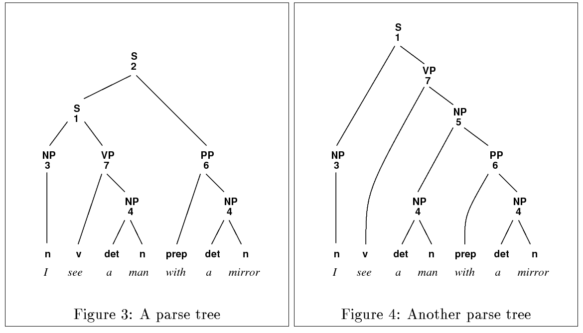
Figure 3: Billot and Lang [1989], Lang [1988]: Ambigious Parse, as Shared Parse Graph
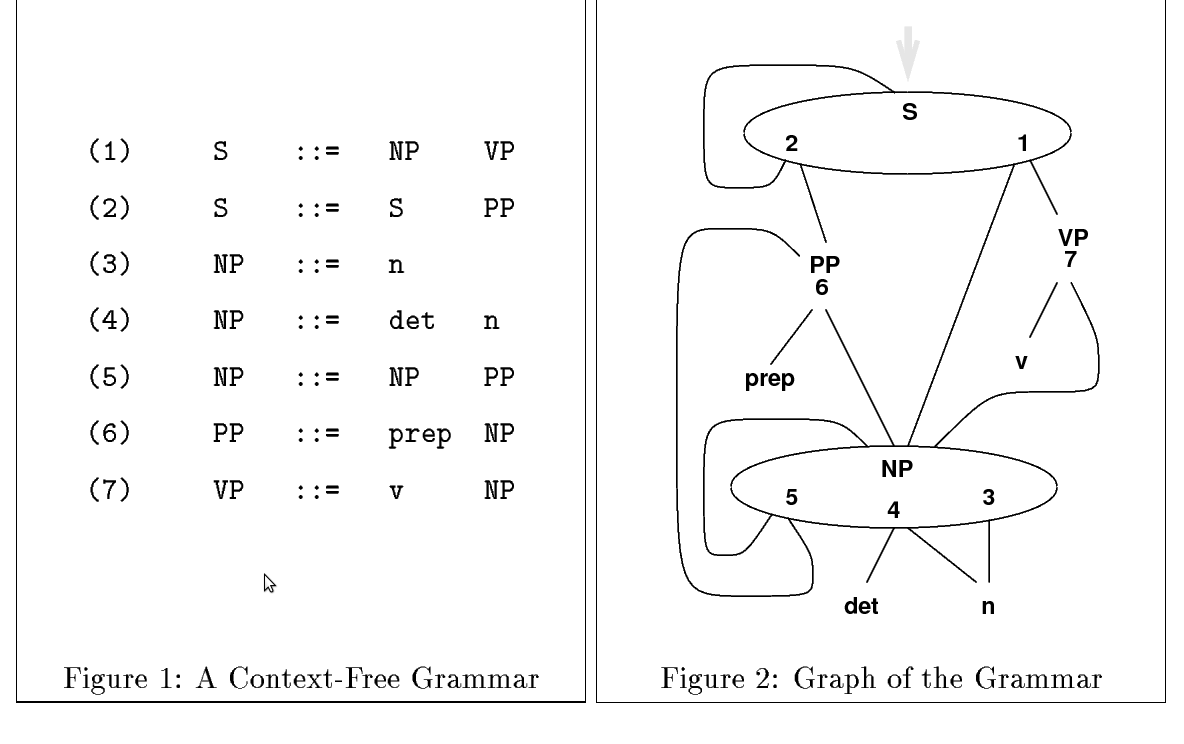
Figure 4: Billot and Lang [1989], Lang [1988]: Ambigious Parse, as Item/Tree Sharing
9 S [Frag(0,2)] → 8 8 VP [Frag(0,2),Wild(2)] → 6,7 7 NP [Frag(0,2)] → 4,5 6 V [Wild(2)] → 3 5 N [Frag(1,2)] → 2 4 D [Frag(0,1)] → 1 3 ’*’ [Wild2] → Term 2 ’boy’ [Frag(1,2)] → Term 1 ’the’ [Frag(0,1)] → Term
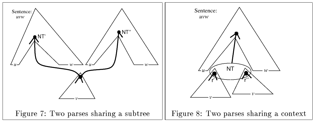
Figure 5: Intersections of Context Free Grammars and Automata
PCFGs have the following properties [Manning et al., 1999]
Our MCFG derivation trees have a context free ’abstract syntax’ [H. Seki and Kasami, 1991, Kallmeyer, 2010]. The MCFG abstract syntax in fact enjoys Place Invariance, Context Freeness, and Ancestor Freeness via its “context-free backbone” [Avarind K. Joshi and Weir., 1992], permitting the extension of PCFG methods to more expressive mildly context sensitive grammars. The parameters for productions in a probabilistic mildly context sensitive grammar can thus be estimated via (Weighted) Relative Frequency Estimation for PCFG [Chi, 1999], as shown in .
| P(A → ξ) = |
| (5) |
Relative Frequency Estimation estimates the likelihood of an outcome by taking a count of the number of outcomes in a data set, and dividing by a count for all contexts in which the event could have had that outcome. For a PCFG G, the event of rewriting a parent A will have outcomes which are rules in G with left hand side A. To estimate the probability of a rule A −> ξ from corpus τ, we only need count the number of occurences of A → ξ in τ as the numerator, and divide by the total number of instances of A as left hand side of a rule in τ.
A PCFG with arbitrary probabilities on productions may fail to define a probabilistic language. For a PCFG G to define a probabilistic language, we require that P be proper and consistent1. Following Chi [1999], a PCFG is proper iff ∑λ:A → ξ) ∈ G P(A → λ) = 1, i.e. for any nonterminal A, the probabilities on rules rewriting A sum to 1. A PCFG G is consistent if ∑x ∈ Σ* P(S ⇒ x) = 1, if the set of all strings derived by G have probabilities summing to 1.
That G is proper is not sufficient to ensure that G defines a probabilistic language. Stolcke [1995] demonstrates a PCFG which is proper but fails to define a probabilistic language, as shown in 6.
2/3 S → S S 1/3 S → ’a’
Figure 6: Inconsistent PCFG
Stolcke [1995] shows that the set of all sentences defined by this probabilistic grammar have probabilities which sum to greater than 1.
for all nonterminals X, the rule probabilities sum to 1
consistent if all string probabilities add to 1.0. = if the PCFG’s fertility matrix 2 A’s spectral radius (largest eigenvalue) ≤ 1.0 = if the fertility matrix A is invertible.
Chi [1999] shows that if a PCFG is trained from a treebank with (Weighted) Relative Frequency Estimation, it is guaranteed to be consistent. The fertility matrix A is indexed by nonterminals, in which the (i,j) entry in A records the expected number of the nonterminal j from one rewriting of the nonterminal i. Grenander [1967], Stolcke [1995] show that the inversion (I−A)−1 gives the transitive closure of the fertility relation; this is crucial for the computation of PCFG entropy and requires a consistent PCFG.
The spectral radius of A shows how recursive the PCFG is; if i(A) ≤ 1.0, then a derivation will halt with certainty. If i(A) ≥ 1.0, then non-terminals are being introduced ’faster’ than they are rewriting into terminals, with the disastrous result that some strings gain infinite probability.
We will need (for several reasons) to compute the inside probability of a category over string or automata. Following Manning et al. [1999, 392], we define the inside probability (βN) of a nonterminal N on an automaton w given a grammar G by 6.
| βN (p,q) = P(wpq|Npq,G) (6) |
Let w(i,j) be an automaton transition sequence between i and j consuming the symbol w. The inside probability βN (p,q) is the probability that a subtree rooted in N has the string yield w(p,q). We typically use dynamic programming via the inside algorithm to compute inside probabilities recursively. For a given nonterminal A, a PCFG G and right hand side ξ, let P(A → ξ|G) be the probability of the rule A → ξ according to G. The inside probability of a nonterminal A is defined inductively:
Base Case: For preterminal nodes A in G, βA (p,q) = P(A → wp,q)|G).
Inductive Case: for other nonterminal nodes A in G, for binary rules of the form A → B1 C1, A → B2 C2..., βA = ∑R(A) ∈ G β(Bi) β(Ci).
Nederhof and Satta [2008] describe the computation of weighted intersection PCFG. Their method obtains the renormalized probability of a situated rule (which we situate wtih indices with (x,y),(x1,y1)...) as a product of the original probability of the unsituated rule and the inside probabilies of situated categories, according to:
| P′(A(x,y)) → B(x1,y1)) = |
| (7) |
| P′(A(x,y) → B(x1,y1)C(x2,y2)) = |
| (8) |
This requires determining the inside probability of a rule, as described in O’Donnell et al. [2009]. Renormalization by inside probability of the branch reflects the true information that an incremental prefix parse contains. To condition a probabilistic context free grammar G on a finite state automata w, we need a weighted intersection G′ whose categories are intersections of categories in G with state transitions in w. The probabilities on productions in G′ need to somehow reflect both probabilities of rules in G and probabilities of state transitions in w.
The inside probability of a category C over a string yield w is the conditional probability of C deriving w given the grammar G and initial probabilities of productions in G. βC moves closer to 0.0 as w|G becomes less likely. Take an example where we have a grammar G with two rules, P A → B1, and P1 A → B2, where P and P1 are the initial probabilities from training. To determine renormalized probabilities P′ and P1′ on the weighted intersection of G and w, P′ should be lowered relative to R′ to the extent that βB1 ≤ βB2. Since the initial probabilities P and P1 are fixed from training, the inside probabilities reflect estimated ’counts’ of rules from w, which drives home the intuitive simularity between the renormalization equations in 7 and 8 and the equation for Relative Frequency Estimation, presented again in 9.
| P(A → ξ) = |
| (9) |
This approach is distinct from pooling probability from rules that do not appear in the intersection directly over to rules that do. Given the previous example, we might set P equal to P + P1 = 1 when A→ B2 fails to appear in the intersection of G and w. Naive renormalization of this type can fail to propogate the information of a string event up through the grammar. When we renormalize by inside probability, we adjust the probabilities of rules whenever the inside probabilities of children non-terminals change. Intuitively, the probability of a rule is reduced whenever any path between the rule and the string yield are eliminated; inside probability propagates this information up to nonterminals higher in the parse. However, naive renormalization reduces the probability of a rule R only when all paths from R are falsified. Naive renormalization overweights many branches because it can adjust probabilities of rules low in the tree without adjusting probabilities of ancestor branches.
For example, renormalization by the inside probability of the branch insures that branches with zero probability and branches with low probability are treated proportionally. Naive renormalization does not insure this because rules only lose probability when they fail to show up in a parse tree, and not when they show up with low probability. An unguarded naive-renormalized derivation admits items to the chart even if those items have zero probability. This could occur, for instance, in the following pathological case, where two rules (D → F,E → G H) are admitted to the training grammar even though they did not show up in treebank.
1.0 100 S → A 0.5 50 A → B C 0.5 50 A → D E 1.0 50 B → F 1.0 50 C → G H 0.0 0 D → F 1.0 50 D → X 0.0 0 E → G H 1.0 50 E → Y 1.0 50 F → ’1’ 1.0 50 G → ’2’ 1.0 50 H → ’3’ 1.0 50 X → ’9’ 1.0 50 Y → ’8’
Figure 7: Pathological Training Example
The unguarded parse of the string ’1 2 3’ incorrectly gives probability to the branch headed by A->D E even though it should have zero probability.
1.0 S → A .5 A → B C .5 A → D E 1.0 B → F 1.0 C → G H 0.0 D → F 0.0 E → G H
Figure 8: Pathological Training Example, Naive Renormalization Without Guards
This occurs because when we parse non-probabilistically, we admit zero probability branches into the parse; when we perform naive renormalization, we eliminate non-present items low in the tree, moving the probability of these eliminated rules to their siblings, but we do not do so high in the tree, because those categories are present in the parse as well.
If we parse with naive renormalization and ’with guards’, by only admitting items to the chart when they have non-zero probability, we sidestep this problem for now.
1.0 S → A 1.0 A → B C 0.0 A → D E 1.0 B → F 1.0 C → G H 0.0 D → F 0.0 E → G H
Figure 9: Pathological Training Example, Naive Renormalization With Guards
We obtain an identical answer if we parse and then renormalize by inside probability.
1.0 S → A 1.0 A → B C 0.0 A → D E 1.0 B → F 1.0 C → G H 0.0 D → F 0.0 E → G H
Figure 10: Pathological Training Example, Renormalization by Inside Probability
Now imagine a less pathological case. The two zero count rules in 7 now have one attestation each in treebank; we adjust the sibling rule counts accordingly.
1.0 100 S → A 0.5 50 A → B C 0.5 50 A → D E 1.0 50 B → F 1.0 50 C → G H 0.02 1 D → F 0.98 49 D → X 0.02 1 E → G H 0.98 49 E → Y 1.0 50 F → ’1’ 1.0 51 G → ’2’ 1.0 51 H → ’3’ 1.0 49 X → ’9’ 1.0 49 Y → ’8’
Figure 11: Less Pathological Example
We again parse the string ’1 2 3’. Naive renormalization without guards still incorrectly leaves the rules with parent A equiprobable.
1.0 S → A .5 A → B C .5 A → D E 1.0 B → F 1.0 C → G H 1.0 D → F 1.0 E → G H
Figure 12: Possible Training Example, Naive Renormalization without Guards
However, naive renormalization with guards still has problems; it does not adjust the probabilities of rules rewriting A because all children of A are attested in the chart, even though some children have very low probabilities.
1.0 S → A .5 A → B C .5 A → D E 1.0 B → F 1.0 C → G H 1.0 D → F 1.0 E → G H
Figure 13: Pathological Training Example, Naive Renormalization with Guards
Renormalizing by inside probability of the branch sidesteps this issue because it always reallocates probabilities whenever any path from non-terminal to child has been falsified.
1.0 S → A 0.996 A → B C 0.004 A → D E 1.0 B → F 1.0 C → G H 1.0 D → F 1.0 E → G H
Figure 14: Possible Training Example, Renormalization by Inside Probability
Thus, renormalization by inside probability of the branch insures that whether zero-probability items are filtered out of the chart or not, we will obtain the same result. Naive renormalization, however, cannot deliver on this guarantee. The difference between 8 and 9 is exactly the problem the parser faces on whether or not to enter zero probability items into the chart. Mcfgcky can emulate naive renormalization, so we tested whether the policy towards parsing non-zero items affected either of naive or inside renormalization. Parsing the prefix “the butter melted *” on unerguacc5.mcfg, we obtained the following entropies:
Without Guards With Guards Naive 4.517 b. 4.431 b. Inside 4.885 b. 4.885 b.
We can conceptualize entropy in terms of a discrete random variable. The entropy of a discrete random variable is equal to −Σi pi log2pi index. A fair coin, for example, has an entropy of −(.5 log .5) + (.5 log .5), i.e., 1.0 bits of entropy, since each of the two possible outcomes (heads, tails) has a 0.5 probability of occurring.
Grenander [1967] demonstrates the computation of entropies of Probabilistic Context Free Grammars. For a PCFG with production rules in Chomsky normal form, let the set of production rules in G be Π, and for a given nonterminal ξ denote the set of rules with parent ξ as Π(ξ)). The entropy associated with a single rewrite of ξ is given by Equation 10
| H(ξ)= −∑r∈Π(ξi) prrlog2pr (10) |
A PCFG is a random process whose outcome is a derivation, and the PCFG’s total entropy is the entropy associated with derivations in Π, where each derivation is a series of rule selection events. Then the entropy of a PCFG is equal to the total entropy of the start symbol S, where the entropy associated with one-step rewrites of ξ must inherit entropy associated with rewriting children of rules in Π(ξ).
Grenander [1967]’s Theorem in Equation 11 provides a recurrence relation for determining the entropy of the start category S; each parent accrues entropy from children weighted by the probabilities of those children.
| H(ξi) = h(ξi) + ∑r∈Π(ξi) pr[H(ξj1) + H(ξj2) + ...] (11) |
The theorem also provides a closed-form solution when the probabilistic context free grammar is recursive or otherwise impractical to compute. The closed-form solution uses linear algebra to efficiently compute the entropy of the hierarchical process in two parts: the ’local’ entropies of parents as simple random variables, and a fertility relation. Let h→ be a vector indexed by nonterminal symbols with each component given by Equation ??.
| hi = h(ξ1) = − |
| prrlog2pr (12) |
Record the one-step fertility relation in a matrix A, labelled with non-terminals, where Ai,j is the expected number of j is the number of i to appear in one rewriting of i. Then the vector of total entropies associated with non-terminals in G is given by Equation 13.
| HG = (I−A)−1 |
| (13) |
For example, the local entropy of a category C according to a pcfg G is the entropy of a die whose sides are labeled and weighted according to one-step rewritings of C. The inversion (I−A)−1 gives the transitive closure of the fertility relation: the expected number of j in a derivation issuing by any number of steps from i. The dot product of right hand side vector h→ and (I−A)−1 gives a vector of total entropies for each non-terminal, including S.